Introduction Dallas Semiconductor uses its unique manufacturing capabilities to provide factory calibrated digital temperature sensors with accuracy as high as ±0.5°C. This level of accuracy is sufficient for many applications; however, some scientific and industrial applications require even greater precision.
This application note presents a technique that can allow the user to improve the accuracy of bandgap-based digital temperature sensors by as much as a factor of 10 by compensating for the offset and curvature of the device error characteristic. This method is successful due the simple second order error curve and the repeatable nature of the output over temperature for bandgap-based sensors.
Note that the technique presented in this article can be applied to any IC temperature sensor with a bandgap-based thermal circuit. This technique will not work for Dallas Semiconductor's older thermal ICs, which have a dual-oscillator-based thermal measurement circuit.
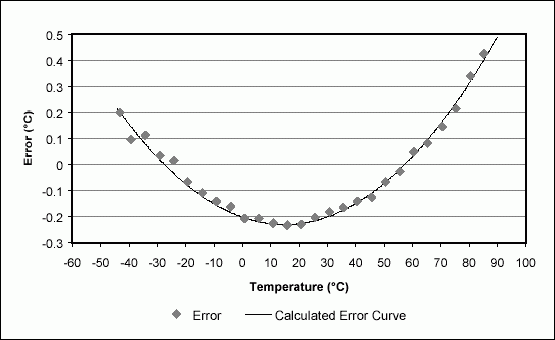
Error Compensation To illustrate the second order error curve inherent to band-gap based sensors, a DS1631 IC was characterized over a -35°C to +85°C temperature range in a thermally conductive liquid bath, and its thermal error relative to a NIST traceable platinum RTD was recorded at 5°C intervals. The results from this sweep are shown in Figure 1 (
 = DS1631 bath measurements).
Figure 1. DS1631 measured error and calculated error.
The error characteristic shown in Figure 1 makes a second order curve that can be represented by the following equation:

where TTS is the temperature measured by the temperature sensor (the DS1631 in this case), α is a curvature correction coefficient, TZERO_SLOPE is the temperature at which the error curve has zero slope, and OFFSET is the error at TZERO_SLOPE.
After determining values for α, OFFSET and TZERO_SLOPE such that Equation 1 provides a close fit to the temperature sensor's output error curve, the user can calculate the approximate measurement error at any temperature and then compensate for the error by subtracting the calculated value from the measured temperature. Thus, the compensated temperature is:

For the best results with this technique, each temperature sensor should be characterized over the desired temperature range in order to determine the best fit calculated error curve for the specific device.
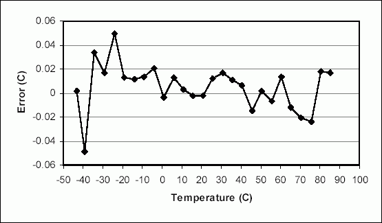
Example This example uses the characterized DS1631 to illustrate the compensation technique described above. Table 1 lists the values measured by the DS1631 and the error of the measurements relative to the actual ambient temperature. From examining Figure 1, TZERO_SLOPE can be estimated to be 15°C and OFFSET to be approximately -0.23°C, for which α = 1.28 x 10⁻⁴ provides a very close fit to the measured error curve (see Figure 1). Plugging the measured temperatures into Equation 2 results in the compensated temperatures shown in Table 1. The error of the compensated temperature relative to the ambient temperature, as shown in Table 1 and Figure 2, is up to 10 times lower than the error of the original measurements.

Figure 2. Example compensated error.
Note that it may take several iterations to arrive at values for TZERO_SLOPE, OFFSET, and α that provide the best fit curve. Once initial estimations for TZERO_SLOPE and OFFSET have been made, α can be calculated with readily available math or spreadsheet software.
Table 1. Compensation example data
欢迎分享,转载请注明来源:内存溢出

 微信扫一扫
微信扫一扫
 支付宝扫一扫
评论列表(0条)